Merging two columns in Excel might sound like a daunting task, but it’s actually pretty simple! All you need to do is use a formula to combine the data from both columns into a new column. You’ll be using the CONCATENATE function or the ampersand (&) to achieve this. Once you’ve merged your columns, you can copy the data and paste it back as values to keep your sheet clean and organized.
Step-by-Step Tutorial for Merging Two Columns in Excel
Let’s dive into the specifics of merging two columns in Excel. You’ll be combining data from two columns into a single column, preserving all the information.
Step 1: Open Your Excel Sheet
Begin by opening the Excel sheet where you want to merge the columns.
Make sure you know which columns you want to merge. For example, if you have first names in column A and last names in column B, you’ll want to combine them into a single column.
Step 2: Choose a Destination Column
Select the cell where you’d like the merged data to appear. This is usually in a new column.
Make sure the destination column is empty to avoid overwriting any existing data. You can use column C if A and B are your merging sources.
Step 3: Enter the Formula
Type the formula =A1 & " " & B1 in the destination cell to merge the data from the first row.
The ampersand (&) acts like glue, sticking your data together with a space in between. You can replace the space with any other delimiter if needed.
Step 4: Drag the Formula Down
Use the fill handle to drag the formula down, applying it to all rows.
This step ensures that the formula is copied down, automatically merging data from each subsequent row.
Step 5: Convert to Values
Highlight the merged column, copy it, then right-click to paste as values.
By pasting as values, you remove the formulas, leaving you with clean, static data that won’t change if you move your original columns.
After completing these actions, you’ll have a new column that combines the data from the two original columns. The original columns remain untouched, so you can keep them for reference or delete them as needed.
Tips for Merging Two Columns in Excel
- Use the CONCATENATE function if you prefer a more formal approach: =CONCATENATE(A1, " “, B1) .
- Always double-check your data for errors before converting formulas to values.
- If merging large datasets, consider splitting the task into smaller sections to avoid mistakes.
- Keep a backup of your original data before merging, just in case.
- Experiment with different delimiters (like commas or dashes) to suit your data presentation needs.
Can I merge more than two columns?
Yes, you can merge as many columns as you like by extending the formula: =A1 & " " & B1 & " " & C1 .
What if my data includes numbers?
The formula works with both text and numbers, merging them seamlessly.
How do I handle empty cells?
If you have empty cells, use the IF function to check for blanks: =IF(A1=”", B1, A1 & " " & B1) .
Can I undo the merge?
Once you paste as values, you can’t directly undo the merge, so keep a backup of your original data.
Will merging affect my existing formulas?
No, merging in a new column won’t impact existing formulas elsewhere in your sheet.
Summary
- Open Excel sheet.
- Choose destination column.
- Enter formula =A1 & " " & B1 .
- Drag formula down.
- Convert to values.
Conclusion
And there you have it! Merging two columns in Excel isn’t as complicated as it seems. By following these simple steps, you can seamlessly combine information, making your data look cleaner and more organized. Whether you’re creating a list of full names or combining product details, these techniques will help you streamline your work.
Excel is a powerful tool, and learning how to use it efficiently can save you loads of time and effort. If you’re dealing with large amounts of data regularly, mastering these skills is worth the investment. Keep exploring and experimenting with different functions and formulas, and you’ll become an Excel wizard in no time.
For more advanced data manipulation, consider learning about Excel’s text functions or exploring pivot tables. The more you learn, the more you’ll realize just how much Excel can do for you. So go ahead, give it a try, and see how merging columns can simplify your spreadsheets today!

Matthew Burleigh has been writing tech tutorials since 2008. His writing has appeared on dozens of different websites and been read over 50 million times.
After receiving his Bachelor’s and Master’s degrees in Computer Science he spent several years working in IT management for small businesses. However, he now works full time writing content online and creating websites.
His main writing topics include iPhones, Microsoft Office, Google Apps, Android, and Photoshop, but he has also written about many other tech topics as well.
Read his full bio here.
Featured guides and deals
Configuring the data in the cells of your Microsoft Excel spreadsheet is often just one part of creating and distributing data. While a spreadsheet may look good on a computer screen, your audience may need a physical copy of the spreadsheet for one reason or another.
Formulas are a very important part of the Excel 2010 user experience because they allow you to automate calculations that need to be performed upon values in Excel. And while the result of those formulas’ calculations is typically the most important part of the equation, you may find yourself in a situation where you need to know how to print formulas in Excel 2010 .
The method for doing so is not very obvious, but it does exist. By following the steps in the tutorial below you will be able to view and print out the formulas that are contained within a cell, as opposed to the calculated value resulting from the formula.
How to Display Formulas in Excel 2010 and Print Them
- Select the Formulas tab.
- Click the Show Formulas button.
- Choose the File tab.
- Select the Print tab.
- Click the Print button.
For additional information on printing formulas in Excel 2010, including pictures of these steps, you can continue to the next section.
Would you like to show some of your data as percentages? Then this guide on how to calculate percentage in Excel can point you in the right direction.
How to Show and Print Excel 2010 Formulas (Guide with Pictures)
There are many different kinds of Excel formulas, and they can be inserted easily as pre-configured formulas, or as formulas that you create yourself. Regardless of their origin, you can change your Excel settings to allow the formulas to be displayed on your screen or when you are printing .
Excel shows the calculated result or calculated values of your formulas by default. It will only be showing formulas if you have set that option for the entire sheet.
Step 1: Open the Excel file containing the formulas that you want to print.
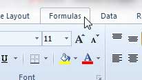
Step 2: Click theFormulastab at the top of the window.
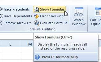
Step 3: Click theShow Formulasbutton in theFormula Auditinggroup section of the ribbon at the top of the window.
Step 4: Click theFiletab at the top-left corner of the window, then click thePrintoption in the column at the left side of the window.
Note that you can also press Ctrl + P on your keyboard to quickly access the Print menu as well.
Step 5: Click thePrintbutton to print the document.
Once the document has been printed with the displayed formulas, you can return to the location identified in Step 3 and click the Show Formulas button again to stop displaying your formulas.
Can I Show or Hide the Formula Bar in Excel?
Above the cells in your spreadsheet is a horizontal section called the formula bar. When Excel is configured to display your formula results in your cells, then you can select a cell to see the formula displayed in the formula bar.
But that formula bar can also be toggled to be shown or hidden, so you might be wondering how to do so.
If you click the View tab at the top of the window you can fin the Formula Bar checkbox in the Show group of the ribbon. Checking or unchecking that box will allow you to hide or display the formula bar at will.
More Information on How to Print Formulas in Excel 2010
The steps above are going to help you to show the formulas in the cells of your spreadsheet, as well as print them out when you print a physical copy of the worksheet.
This is a common request when you are working with Excel in a computer class or another learning or scholastic environment. An important part of learning to use Excel is properly incorporating formulas and functions into your workflow. Many people who are new to Excel or intimidated by it will perform their calculations on a calculator, or won’t use the tools within the application to generate results. If someone is asking you to show and print your formulas then they want to see that you arrived at a solution using a formula, rather than simply typing the desired result into the cell.
Excel is going to expand the width of your columns a bit when you enable the “Show Formulas” option, but it may not be enough to fully display the formulas. You can double-click the right column heading border to automatically expand its width and show the widest data within the column.
If you select the Page Layout tab at the top of the window you can click the small Page Setup button that is located at the bottom-right of the Page Setup group of the ribbon. This is going to open the Page Setup dialog box where you can adjust various settings that will affect the appearance of your printed page. You can adjust various print settings for the worksheet including options like choosing to print titles, or the page order if you will have multiple pages when you choose to print active sheets.
You could also click the Print Preview button to see how your spreadsheet will look if you have elected to display formulas or calculated results. On the Print menu you can also adjust options like whether to print active sheets or the entire Excel workbook. You can also switch the page orientation, or you can modify the scaling so that all the columns or all the rows fit on one page.
If you open the Page Layout tab you will find a Sheet Options group where you can elect to view or print column headings or gridlines.
When you need to print multiple worksheets but not the entire workbook then you can hold down the Ctrl key on your keyboard and click each of the sheet tabs that you want to include in the print job.
Are you finding that your formulas aren’t updating when you change a value that should change a formula result? Find out how to force Excel to calculate your formulas by enabling an automatic calculation option.
Matthew Burleigh has been writing tech tutorials since 2008. His writing has appeared on dozens of different websites and been read over 50 million times.
After receiving his Bachelor’s and Master’s degrees in Computer Science he spent several years working in IT management for small businesses. However, he now works full time writing content online and creating websites.
His main writing topics include iPhones, Microsoft Office, Google Apps, Android, and Photoshop, but he has also written about many other tech topics as well.
Read his full bio here.
